Deriving The Homfly Polynomial From The Braid Groups

Braids have many useful applications to knot theory. Consider taking a geometric braid and identifying the beginning and endings of its strands (in order) to create a closed braid. This closed braid will be a link. In fact, in 1923 James Alexander proved that every link can be represented by a closed braid. This discovery was made even more useful by a result of Markov which relates equivalence of links to equivalence of braids. Two braids are $M$-equivalent if they can be transformed into each other in the braid group and with the additional following two rules (called Markov moves). The first new rule, sometimes called conjugation, is that given $b_1, b_2 \in B_n$, $b_1 \mapsto b_2 b_1 b_2^{-1}$. The second new rule is that for $b_1 \in B_n$, $b_1 \mapsto \sigma_n^{\pm 1}\iota( b_1)$ where $\iota: B_n \to B_{n+1}$ is the inclusion map. These two rules form an equivalence relation $\sim$ on $B = \bigcup_{n \geq 1} B_n$ such that $B/\sim$ is isomorphic to the space of links in $\mathbb{R}^3$. This is discussed in more detail in (Adams, 1994).

This strong connection between links and braids has led to numerous results in knot theory including the Alexander, Jones, and HOMFLY polynomials, as well as solutions for recognizing the unknot. The HOMFLY polynomial is a link invariant discovered in 1985 by Hoste, Ocneanu, Millett, Freyd, Lickorish, and Yetter (hence HOMFLY). It is a two variable generalization of the Jones and Alexander polynomials. Here we explore the construction of the HOMFLY polynomial from the braid groups and outline the proof for it being a link invariant. Our construction is based on material from (Kassel, 2008).

Using the rules for $M$-equivalence, we can define a special type of function which must provide an invariant on links.

A set of maps $\{f_n : B_n \to E\}_{n\geq 1}$ is a Markov function if it has the properties: 1. For any $n\geq 1$ and $b_1, b_2 \in B_n$, $f_n(b_1 b_2) = f_n(b_2 b_1)$ 2. For any $n\geq 1$ and $b \in B_n$, $f_n(b) = f_{n+1}(\sigma_n b)$ and $f_n(b) = f_{n+1}(\sigma_n^{-1} b)$.

The first criteria to be a Markov function ensures that the value of the function is invariant under conjugation. The second criterion ensures that the function is invariant under the second rule for $M$-equivalence. Given a Markov function $f$ a link invariant can be defined in the following way. Let $L$ be a link and let $b$ be a braid whose closed form is isotopy equivalent to $L$. Then define $\hat{f}(L) = f(b)$. Since $f$ is invariant under Markov moves, given two distinct braids $b_1$ and $b_2$ whose closed forms are isotopy equivalent to $L$, $f(b_1) = f(b_2)$. Therefore $\hat{f}$ is an invariant on links. By defining explicit Markov functions we can create new knot invariants. Constant functions satisfy the conditions for being a Markov function, but they are not a very interesting example. To construct a more interesting Markov function, we define the Iwahori Hecke Algebras. The Iwahori Hecke algebras share some structure with the braid groups and elements of the braid group can be mapped to corresponding elements in an Iwahori Hecke Algebra by a canonical map $w: B_n \to H^R_n(q,z)$. Finally, we define a trace operator $tr_n: H_n \to R$ (the Ocneanu traces) on the Iwahori Hecke Algebras and show that $tr_n \circ w$ is a Markov function. This function is the HOMFLY polynomial.

Algebraic Background

A few algebra preliminaries are necessary to understand the construction of the HOMFLY polynomial.

Let $R$ be a ring with multiplicative identity $1_R$. A module over $R$, or an $R$-module, is similar to a vector space over a field $F$.

A left $R$-module $M$ is an abelian group $(M, +)$ with a scalar multiplication $\cdot : R \times M \to M$ with the following properties for all $a, b \in R$ and $x, y \in M$: 1. $\cdot$ is distributive over addition in both arguments: \[ a \cdot (x + y) = a \cdot x + a \cdot y \text{ and } (a+b) \cdot x = a \cdot x + b \cdot y, \] 2. Multiplication is associative: \[ (ab) \cdot x = a \cdot (b \cdot x), \text{ and}\] 3. $1_R$ is the multiplicative identity in the module, \[1_R \cdot x = x.\] A right module is defined by making scalar multiplication act on the right instead of the left, i.e. $\cdot: M \times R \to M$. If $M$ is both a right and left $R$-module and $(r_1 m) r_2 = r_1 (m r_2)$ for all $r_1, r_2 \in R$ and $m \in M$ then $M$ is a $R$-bimodule (or just an $R$-module). If $R$ is commutative then any $R$-module will be a bimodule.

If $R$ is a field then an $R$-module is just a vector space over $R$.

The set of infinitely differentiable functions from $\mathbb{R}^3 $ to $\mathbb{R}$ form a ring $C^\infty(\mathbb{R}^3)$ under pointwise addition and multiplication (but not a field). Let $\mathfrak{X}(\mathbb{R}^3)$ be the set of all vector fields on $\mathbb{R}^3$. For any $X, Y \in \mathfrak{X}(\mathbb{R}^3)$ and $p \in \mathbb{R}^3$ define \[(X + Y)(p) = X(p) + Y(p).\] This addition forms an abelian group $( \mathfrak{X}(\mathbb{R}^3), +)$. If $f \in C^\infty(\mathbb{R}^3)$ is an infinitely differentiable function on $\mathbb{R}^3$ then \[(fX)(p) = f(p)X(p)\] for any $p \in \mathbb{R}^3$ defines a scalar multiplication and turns $\mathfrak{X}(\mathbb{R}^3)$ into a $C^\infty(\mathbb{R}^3)$-module. We use this module in vector calculus even without explicitly defining it.

Just like a vector space has a basis, modules can also have a basis (although they may not). Let $M$ be an $R$-module. A set $E \subset M$ is a basis for $M$ if $E$ is a generating set for $M$ and $E$ is linearly independent. A free module is a module with a basis.

The concept of a bilinear map is important for defining the tensor product of $R$-modules. A bilinear map extends the notion of a linear map to maps of two variables by making the map linear on each variable. Let $X, Y, Z$ be $R$-Modules and $f : X \times Y \to Z$ be a mapping. $f$ is bilinear if it has the properties that for all $x, x’ \in X$, $y, y’ \in Y$ and $r \in R$,

\[f(x + x', y) = f(x, y) + f(x', y),\] \[f(x, y+y') = f(x, y) + f(x, y')\] \[f(r \cdot x, y) = rf(x, y) = f(x, r \cdot y)\]

That is, for fixed $x \in X$, $f_x = f(x, -)$ is a linear map and for fixed $y \in Y$, $f_y = f(-, y)$ is a linear map.

Let $M$ and $N$ be $R$-modules, $\otimes_R : M \times N \to M \otimes_R N$ is a bilinear map which takes $(m, n) \mapsto m \otimes_R n$ with the property that for every abelian group $G$ and every bilinear map $f: M \times N \to G$ there is a unique $R$-module homomorphism $\hat{f}: M \otimes_R N \to G$ such that this diagram commutes:

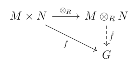
In fact, this property defines a unique space $M \otimes_R N$. If $M$ and $N$ are free $R$-modules of dimension $k$ and $l$ resp. with bases $(m^i)_{1 \leq i \leq k}$ and $(n^j)_{1 \leq i \leq l}$, then $M \otimes_R N$ is a free $R$-module of dimension $kn$ with a basis given by $(m^i \otimes_R n^j)_{1 \leq i \leq k, 1 \leq i \leq l}$. Free modules and their tensor products are used to construct the HOMFLY polynomial.

Let $V$ be a real vector space. The dual space $V^*$ of $V$ is defined as the set of all linear functionals from $V$ to $\mathbb{R}$. Under pointwise addition and scalar multiplication, $V^*$ is itself a vector space. Let $v*, w^* \in V^*$. Consider the map $\psi : V^* \otimes V^* \to (V \times V)^*$ defined by \[\phi(v^* \otimes u^*)(a, b) = v^*(a)u^*(b).\] This map allows us to view $v^* \otimes u^*$ as a bilinear functional on $V \times V$. We can use these tensor products of dual vectors in linear algebra. For example, if $v^* \otimes u^*$ is non-degenerate and positive-semidefinite $v^* \otimes u^*$ defines an inner product on $V$.

Let $A$ be an $R$-Module with a bilinear multiplication map $A \times A \to A$ on $A$ such that:

For any $x, y, z \in A$, $x(yz) = xyz = (xy)z$,
For any $a \in R$ and any $x, y \in A$, $a \cdot (xy) = (a \cdot x)y = x(a \cdot y)$, and
There exists $1 \in A$ such that for all $x \in A$, $1x = x = x1$.

Then $A$ is an associative $R$-algebra.

The Iwahori Hecke Algebras

Let $R$ be a fixed commutative ring and $q, z \in R$ be fixed. Then the Iwahori Hecke Algebra $H_n = H_n^R(q, z)$ is an associative $R$-algebra with multiplicative unity $1$, generators $T_1, T_2, ..., T_{n-1}$ and relations 1. $T_i T_j = T_j T_i$ for $|i - j| \geq 2$, 2. $T_i T_{i+1} T_i = T_{i+1} T_i T_{i+1}$ for $i = 1, 2, ..., n-2$, and 3. $T_i^{-1} = q^{-1}(T_i - z1)$ for $i = 1, 2, ..., n-1$.

The first two relations of the Iwahori Hecke algebra are the same as the relations for the braid group, but the third relation is new. Take any product of these generators

\[w = \prod_{i_j} T_{i_j}\]

where $(i_j)$ is a finite sequence of indices. We will call these “words.” All elements in $H_{n+1}$ can be written as a finite sum of words with $i_j = 1, 2, … n$. Let $\lambda(w)$ be the number of generators in $w$ (i.e. the length of the word).

Let $\iota : H_n \to H_{n+1}$ be a map defined on the generators of $H_n$ by $T_i \mapsto T_i$ for $i = 1, …, n-1$. Then $\iota(w)h$ for $w \in H_{n-1}$ and $h \in H_n$ defines a multiplication operation which turns $H_n$ into a left $H_{n-1}$-module. Let $T’ = {1, T_n, T_n T_{n-1}, …, T_n T_{n-1} … T_2 T_1}$. We claim that it is possible to write any word $w$ in the form $\iota(\tilde{w}) t’$ where $\tilde{w}$ is a word in $H_{n}$ and $t’ \in T’$, or as a sum of words in this form. Let $t_k = T_n T_{n-1} … T_{k}$.

Suppose $w = \iota(a) t_k T_i b$ for $a \in H_n$, $b \in H_{n+1}$ and $T_i$ any generator of $H_{n+1}$. If $w$ has no adjacent generators the following hold: 1. If $k - i > 1$, then $w = \iota(a) T_i t_k b$; 2. If $i = k-1$, then $w = \iota(a) t_{k-1} b$; and 3. If $n \geq i \geq k$, $w = \iota(a) T_{i-1} t_k b$.

If $| i - k | > 1$, then $T_i$ commutes with $T_k, T_{k+1}... T_n$ and it follows that $w = \iota(a) t_k T_i b = \iota(a) T_i t_k b$. If $i = k-1$ then $w = \iota(a) t_k T_i b = \iota(a) t_{k-1} b$ by definition of $t_\cdot$. If $n \geq i \geq k$ then $w = \iota(a) t_k T_i b $$= \iota(a) T_n T_{n-1} ... T_i T_{i-1} ... T_{k} T_i b$ $= \iota(a) T_n T_{n-1} ... T_i T_{i-1} T_i... T_{k} b$ $= \iota(a) T_n T_{n-1}... T_{i-1} T_i T_{i-1} ... T_{k} b$ $= \iota(a) T_{i-1} T_n T_{n-1} ... T_{k} b$ $= \iota(a) T_{i-1} t_k b$.

Let $w$ be a word in $H_{n+1}$ of length $l$ with no adjacent generators (i.e. $T_i T_i$). If $w \not \in H_{n}$ then $w = \iota(a) T_n b_0$ for $a \in H_{n}$ and $b_0 = T_{i_j} b_{1} \in H_{n+1}$. Suppose that $w = \iota(a) t_k b_j$ for some $k = 1, 2, … n$, $a \in H_{n}$ and $b_j = T_{i_j} b_{j+1} \in H_{n+1}$. Since $w$ has no adjacent generators, either $k - i_j = 1$, $k - i_j > 1$ or $n \geq i_j \geq k$. Therefore by the previous Lemma, if $k - i_j = 1$ then $w = \iota(a) T_{i_j} t_k b_{j+1}$. If $k - i_j > 1$ then $w = \iota(a) t_{k-1} b_{j+1}$. If $n \geq i \geq k$, $w = \iota(a) T_{i_j-1} t_k b_{j+1}$. In any case, the length of the word after the segment in the required form is decreased by 1 (i.e. $\lambda(b_{j+1}) = \lambda(b_{j}) - 1$). By induction on $j$, $w$ can be rewritten in $m$ steps such that the length of the word after the segment in the required form is $\lambda(b_0) - m$ for $m \leq \lambda(b_0)$. Therefore, $w$ can be rewritten into the desired form in $O(l)$ time.

The third relation of the Iwahori Hecke Algebras says that any $T_i^m = c_1(m) T_i + c_2(m)$ where $c_1(m)$ and $c_2(m)$ are in $R$ and depend on $m$. Therefore we can expand any word $w \in H_{n+1}$ into a sum of words with no adjacent generators and then the algorithm gives a sum of words in the form $\iota(\tilde{w}) t_k$ where $t_k \in T’$ and $w \in H_n$. Since $T’$ is linearly independent, we obtain the following consequence.

1
$H_n$ is a free $H_{n-1}$-module with a basis $\{1, T_{n-1}, T_{n-1}T_{n-2} ..., T_{n-1}T_{n-2} ... T_2 T_1\}$ and $\iota: H_{n-1} \to H_n$ is an injective homomorphism.

See the above discussion and algorithm or the proof of Proposition 4.21 in (Kassel, 2008).

2
There is a $H_n$-module isomorphism \[\phi_n: H_n \oplus (H_n \otimes_{H_{n-1}} H_n) \to H_{n+1}\] defined by \[(x + \sum_i y_i \otimes z_i) \mapsto \iota(x) + \sum_i y_i T_n z_i\] for any $x \in H_n$, $\sum_i y_i \otimes z_i \in H_n \otimes_{H_{n-1}} H_n$.

We use the universal property of tensor product spaces to show that this mapping is a well defined homomorphism on elements in $H_n \otimes_{H_{n-1}} H_n$. Let $f : H_n \times H_n \to H_{n+1}$ be defined by $(a, b) \mapsto aT_nb$. Since $T_i T_j = T_j T_i$ for $|i - j| \geq 2$, for any $h \in H_{n-1}$ and $a, b, c\in H_n$, \[f(ah, b) = ahT_nb = aT_n h b = f(a, hb),\] \[f(a+c, b) = (a+c)T_n b = aT_nb + cT_nb = f(a,b)+f(c, b), \text{ and}\] \[f(a, b+c) = aT_n(b+c) = aT_nb + aT_nc = f(a,b)+f(a,c).\] Therefore $f$ is a bilinear map and defines a unique module homomorphism $\tilde{f}: H_n \otimes_{H_{n-1}} H_n \to H_{n+1}$ such that $\tilde{f} \circ \otimes_{H_{n-1}} = f$. Since \[(\phi_n \circ \otimes_{H_{n-1}}) (a, b) = \phi(a \otimes b) = aT_nb,\] $\tilde{f} = \phi$ and $\phi$ is a well-defined module homomorphism on the elements $a \otimes b$. This extends to $H_n \oplus (H_n \otimes_{H_{n-1}} H_n)$ since $\iota$ is a module homomorphism. As a $H_{n-1}$-module $H_n \oplus (H_n \otimes_{H_{n-1}} H_n)$ has a basis given by \[\{T_{n-1}, T_{n-1}T_{n-2},...\} \coprod \{1 \otimes 1, T_{n-1} \otimes 1, T_{n-1} T_{n-2} \otimes 1, ...\] \[T_{n-1} \otimes T_{n-1}, ..., T_{n-1}T_{n-2}...T_2 T_1 \otimes T_{n-1}T_{n-2}...T_2 T_1 \}.\] If instead we look at $H_n \oplus (H_n \otimes_{H_{n-1}} H_n)$ as an $H_n$ module, this basis reduces to \[\{1\} \coprod \{ 1 \otimes 1, 1 \otimes T_{n-1}, 1 \otimes T_{n-1}T_{n-2}, ... 1 \otimes T_{n-1}T_{n-2}...T_2 T_1\}.\] $\phi_n$ sends this basis to $\{1, T_n, T_n T_{n-1}, ...T_n T_{n-1}...T_2 T_1\}$ which by Theorem 1 is the basis for $H_{n+1}$ as an $H_n$ module. Therefore $\phi_n$ is a $H_n$-module isomorphism.

This theorem also implies that $\phi$ is an R-module since every $r \in R$ is in $H_n$. Therefore $\phi$ is an $R$-module homomorphism and still bijective.

Ocneanu Trace

This isomorphism is used to define the Ocneanu trace $tr_n: H_n \to R$. The trace is defined inductively on $n$. For the case $n=1$, $H_1$ has basis ${1}$ and so $H_1 = R$. Therefore we can define $tr_1 = Id_R$ to be the identity map on $R$. For $n=2$ the basis for $H_2$ is ${1, T_1}$. In general, we would like $tr_2 \circ w$ on the unknot to be 1. Since the closed form of $\sigma_1$ is the unknot and $w(\sigma_1) = T_1$, we define

\[tr_2(T_1) = 1 \text{ and } tr_2(1) = \frac{1-q}{z}.\]

For $n\geq 2$, assume $tr_n : H_n \to R$ is a well defined $R$-linear function (i.e. $tr_n(ra) = rtr_n(a)$ for all $r \in R$ and $a \in H_n$). Then $tr_{n+1}$ is defined using inductively using $\phi_n$. For $a, b, c \in H_n,$

\[tr_{n+1}(\phi_n(a)) = \frac{1-q}{z} tr_n(a) \text{ and } tr_{n+1}(\phi_n(b \otimes_{H_{n-1}} c)) = tr_n(bc).\]

$tr_{n+1}$ is $R$-linear since $\phi$, $tr_n$, and $\otimes_{H_{n-1}}$ are.

For all $a, b \in H_n$ and $n\geq 1$, 1. $tr_n(ab) = tr_n(ba)$, and 2. $tr_{n+1}(T_n a) = tr_{n+1}(T_n^{-1} a) = tr_n(a)$.

(1) The proof that $tr_n(ab) = tr_n(ba)$ is done by induction on $n$. For $n=1$ and $n=2$ this is true because $H_1$ and $H_2$ are commutative. Suppose this relation is true for $tr_n$. $H_{n+1}$ is generated by $T_1, ..., T_n$ and $\phi_n$ is onto, so it suffices to show that $tr_{n+1}(wT_i) = tr_{n+1}(T_i w)$ for all $w \in \text{im} \phi_n$ and $i = 1, ..., n$. Suppose $w = \phi(a)$ for an $a \in H_n$. If $i < n$, then $tr_{n+1}(wT_i) = \frac{1- q}{z} tr_n(aT_i)$ and $tr_{n+1}(T_i w) = \frac{1- q}{z} tr_n(T_i a)$ which are equal from the induction hypothesis. If $i=n$, then $tr_{n+1}(wT_n) = tr_n(a)$ and $tr_{n+1}(T_nw) = tr_n(a)$. Suppose $w = \phi(a \otimes_{H_{n-1}} b) = a T_n b$ for $a, b \in H_n$. If $i < n$, then $bT_i \in H_n$ and $aT_n b T_i = \phi(a \otimes b T_i)$. Therefore, \begin{align*} tr_{n+1}(wT_i) & = tr_{n+1}(a T_n b T_i) \\ & = tr_{n+1}(\phi_n(a \otimes b T_i)) = tr_n(abT_i) \\ & = tr_n(T_i ab) = tr_{n+1}(T_i w) \end{align*} If $i = n$ then there are four possible cases. If $a, b \in H_{n-1}$ then $T_n$ commutes with both and $T_n ab = ab T_n$ implies the property. If only $a \in H_{n-1}$, then $b = \phi_{n-1}(c \otimes d) = cT_{n-1} d$ for some $c, d \in H_{n-1}$. Then $a, c$ and $d$ commute with $T_n$. Therefore, \begin{align*} tr_{n+1}(aT_n b T_n) &= tr_{n+1}(a T_n c T_{n-1} d T_n) \\ & = tr_{n+1}(a c T_n T_{n-1} T_n d ) = tr_{n+1}(a c T_{n-1} T_n T_{n-1} d ) \\ & = tr_{n+1}(\phi_n(a c T_{n-1} \otimes T_{n-1} d)) = tr_n(ac T^2_{n-1} d) \\ & = ztr_n(acT_{n-1} d) + q tr_n(acd) \\ & = z tr_n(ab) + q\frac{1-q}{z} tr_{n-1}(a c d) \end{align*} and \begin{align*} tr_{n+1}(T_naT_nb) &= tr_{n+1}(T_n^2 a b) \\ & = ztr_{n+1}(T_n ab) + qtr_{n+1}(ab) \\ & = ztr_n(ab) + q \frac{1 -q}{z} tr_n(a c T_{n-1} d) \\ &= z tr_n(ab) + q \frac{1 -q}{z} tr_{n-1}(acd). \end{align*} Therefore $tr_{n+1}(aT_n b T_n) = tr_{n+1}(T_naT_nb)$. If only $b \in H_{n-1}$, the proof is similar to the previous case. If neither of $a, b \in H_{n-1}$ then $a = \phi_{n-1}(e \otimes f) = eT_{n-1} f$ and $b = \phi_{n-1}(c \otimes d) = cT_{n-1} d$ for some $c, d, e, f \in H_{n-1}$. $c, d, e,$ and $f$ all commute with $T_n$. Then \begin{align*} tr_{n+1}(a T_n b T_n) &= tr_{n+1}(a T_n c T_{n-1} d T_n) \\ & = tr_{n+1}(ac T_n T_{n-1} T_n d) \\ & = tr_{n+1}(ac T_{n-1} T_n T_{n-1} d) = tr_{n+1}(\phi_n(ac T_{n-1} \otimes T_{n-1} d)) \\ & = tr_n(ac T_{n-1}^2 d) \\ & = ztr_n(acT_{n-1}d) + q tr_n(a c d) \\ & = ztr_n(ab) + q tr_n(e T_{n-1} f c d ) = ztr_n(ab) + q tr_n(\phi_{n-1}(e \otimes f c d) ) \\ &= ztr_n(ab) + q tr_n(e f c d) \end{align*} and \begin{align*} tr_{n+1}(T_n a T_n b) &= tr_{n+1}(T_n e T_{n-1} f T_n b) \\ &= tr_{n+1}(e T_n T_{n-1} T_n fb) \\ &= tr_{n+1}(e T_{n-1} T_n T_{n-1} fb) = tr_{n+1}(\phi_n( e T_{n-1} \otimes T_{n-1} fb ))\\ &= tr_n(e T_{n-1}^2 fb) \\ & = ztr_n(e T_{n-1} f b) + q tr_n(e f b) \\ & = ztr_n(ab) + q tr_n(ef c T_{n-1} d) = ztr_n(ab) + q tr_n(\phi_{n-1}(ef c \otimes d)) \\ & = ztr_n(ab) + q tr_{n-1}(ef c d). \end{align*} These expressions are identical, therefore $tr_{n+1}(a T_n b T_n) = tr_{n+1}(T_n a T_n b).$ By induction this property holds for all $n \geq 1$. (2) For all $a \in H_n$, \[ tr_{n+1}(T_n a) = tr_{n+1}(\phi_n(1 \otimes a)) = tr_n(a). \] From the third relation on the Iwahori-Hecke algebra, $T_n^{-1} = q^{-1}(T_n - z1)$. Therefore, \begin{multline*} tr_{n+1}(T^{-1}_n a) = q^{-1}tr_{n+1}( T_na - z1a) \\ = q^{-1}(tr_{n+1}( T_na) - ztr_{n+1}(a))) \\ = q^{-1}(tr_n(a) - z\frac{1-q}{z}tr_n(a)) = tr_n(a). \end{multline*} Therefore $tr_{n+1}(T_n a) = tr_{n+1}(T_n^{-1} a) = tr_n(a)$.

HOMFLY Polynomial

This theorem shows that if $w_n: B_n \to T_n$ is defined by $\sigma_i \mapsto T_i$, then $tr_n \circ w_n$ is a Markov function. Therefore this defines an invariant for links which is parameterized by $q$ and $z$. For any link $L$, let $b \in B_n$ be a braid whose closed form is isotopic to $L$. Then $I_L(q, z) = tr_n(w_n(b)) \in R$ depends only on the isotopy class of $L$. The closure of the trivial braid $1$ is the unknot. Therefore for the unknot, $I_{\text{unknot}}(q, z) = tr_1(w_1(1)) = tr_1(1) = 1$.

Let $R = \mathbb{Z}[x, x^{-1}, y, y^{-1}]$ and set $P_L(x, y) = I_L(q, z)$ for $q = x^{-2}$ and $z=x^{-1}y$. From the preceding paragraph, we know that $P_L(x,y)$ is a link invariant and that $P_{\text{unknot}}(x, y) = 1$. $P_L(x, y)$ is the HOMFLY polynomial.

References

Adams, C. (Colin C. (1994). The knot book: An elementary introduction to the mathematical theory of knots. W.H. Freeman.

BIRMAN, J. S., & Cannon, J. (1974). Braids, Links, and Mapping Class Groups. (AM-82). Princeton University Press. http://www.jstor.org/stable/j.ctt1b9rzv3

Kassel, C. (2008). Braid Groups (1st ed. 2008.). Springer New York : Imprint: Springer.

Written on August 2, 2020